Plot the optimal encoding
# S3 method for class 'fmca'
plot(
  x,
  harm = 1,
  states = NULL,
  addCI = FALSE,
  coeff = 1.96,
  col = NULL,
  nx = 128,
  ...
)
Arguments
- x
output of
compute_optimal_encodingfunction- harm
harmonic to use for the encoding
- states
states to plot (default = NULL, it plots all states)
- addCI
if TRUE, plot confidence interval (only when
computeCI = TRUEincompute_optimal_encoding)- coeff
the confidence interval is computed with +- coeff * the standard deviation
- col
a vector containing color for each state
- nx
number of time points used to plot
- ...
not used
Value
a ggplot object that can be modified using ggplot2 package.
Details
The encoding for the harmonic h is \(a_{x}^{(h)} \approx \sum_{i=1}^m \alpha_{x,i}^{(h)}\phi_i\).
See also
Other encoding functions:
compute_optimal_encoding(),
get_encoding(),
plotComponent(),
plotEigenvalues(),
predict.fmca(),
print.fmca(),
summary.fmca()
Examples
# Simulate the Jukes-Cantor model of nucleotide replacement
K <- 4
Tmax <- 6
PJK <- matrix(1 / 3, nrow = K, ncol = K) - diag(rep(1 / 3, K))
lambda_PJK <- c(1, 1, 1, 1)
d_JK <- generate_Markov(n = 10, K = K, P = PJK, lambda = lambda_PJK, Tmax = Tmax)
d_JK2 <- cut_data(d_JK, Tmax)
# create basis object
m <- 6
b <- create.bspline.basis(c(0, Tmax), nbasis = m, norder = 4)
# \donttest{
# compute encoding
encoding <- compute_optimal_encoding(d_JK2, b, computeCI = FALSE, nCores = 1)
#> ######### Compute encoding #########
#> Number of individuals: 10
#> Number of states: 4
#> Basis type: bspline
#> Number of basis functions: 6
#> Number of cores: 1
#> Method: precompute
#>
| | 0 % elapsed=00s
|========= | 17% elapsed=00s, remaining~00s
|================= | 33% elapsed=00s, remaining~00s
|========================= | 50% elapsed=00s, remaining~00s
|================================== | 67% elapsed=00s, remaining~00s
|========================================== | 83% elapsed=00s, remaining~00s
|==================================================| 100% elapsed=00s, remaining~00s
#>
#> DONE in 0.09s
#> ---- Compute U matrix:
#>
| | 0 % elapsed=00s
|=== | 5 % elapsed=00s, remaining~00s
|===== | 10% elapsed=00s, remaining~00s
|======== | 14% elapsed=00s, remaining~00s
|========== | 19% elapsed=00s, remaining~00s
|============ | 24% elapsed=00s, remaining~00s
|=============== | 29% elapsed=00s, remaining~00s
|================= | 33% elapsed=00s, remaining~00s
|==================== | 38% elapsed=00s, remaining~00s
|====================== | 43% elapsed=00s, remaining~00s
|======================== | 48% elapsed=00s, remaining~00s
|=========================== | 52% elapsed=00s, remaining~00s
|============================= | 57% elapsed=00s, remaining~00s
|=============================== | 62% elapsed=00s, remaining~00s
|================================== | 67% elapsed=00s, remaining~00s
|==================================== | 71% elapsed=00s, remaining~00s
|======================================= | 76% elapsed=00s, remaining~00s
|========================================= | 81% elapsed=00s, remaining~00s
|=========================================== | 86% elapsed=00s, remaining~00s
|============================================== | 90% elapsed=00s, remaining~00s
|================================================ | 95% elapsed=00s, remaining~00s
|==================================================| 100% elapsed=00s, remaining~00s
#>
| | 0 % ~calculating
|===== | 10% ~00s
|========== | 20% ~00s
|=============== | 30% ~00s
|==================== | 40% ~00s
|========================= | 50% ~00s
|============================== | 60% ~00s
|=================================== | 70% ~00s
|======================================== | 80% ~00s
|============================================= | 90% ~00s
|==================================================| 100% elapsed=00s
#>
#> DONE in 0.47s
#> ---- Compute encoding:
#> DONE in 0s
#> Run Time: 0.58s
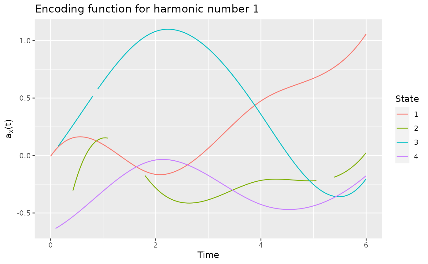
# plot the encoding produced by the first harmonic
plot(encoding)
#> Warning: Removed 14 rows containing missing values or values outside the scale range
#> (`geom_line()`).
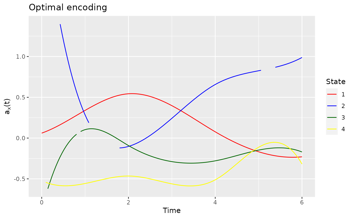
 # modify the plot using ggplot2
library(ggplot2)
plot(encoding, harm = 2, col = c("red", "blue", "darkgreen", "yellow")) +
labs(title = "Optimal encoding")
#> Warning: Removed 14 rows containing missing values or values outside the scale range
#> (`geom_line()`).
# modify the plot using ggplot2
library(ggplot2)
plot(encoding, harm = 2, col = c("red", "blue", "darkgreen", "yellow")) +
labs(title = "Optimal encoding")
#> Warning: Removed 14 rows containing missing values or values outside the scale range
#> (`geom_line()`).
 # }
# }