Plot Eigenvalues
plotEigenvalues(x, cumulative = FALSE, normalize = FALSE, ...)Arguments
- x
output of
compute_optimal_encodingfunction- cumulative
if TRUE, plot the cumulative eigenvalues
- normalize
if TRUE eigenvalues are normalized for summing to 1
- ...
geom_pointparameters
Value
a ggplot object that can be modified using ggplot2 package.
See also
Other encoding functions:
compute_optimal_encoding(),
get_encoding(),
plot.fmca(),
plotComponent(),
predict.fmca(),
print.fmca(),
summary.fmca()
Examples
# Simulate the Jukes-Cantor model of nucleotide replacement
K <- 4
Tmax <- 6
PJK <- matrix(1 / 3, nrow = K, ncol = K) - diag(rep(1 / 3, K))
lambda_PJK <- c(1, 1, 1, 1)
d_JK <- generate_Markov(n = 10, K = K, P = PJK, lambda = lambda_PJK, Tmax = Tmax)
d_JK2 <- cut_data(d_JK, Tmax)
# create basis object
m <- 6
b <- create.bspline.basis(c(0, Tmax), nbasis = m, norder = 4)
# \donttest{
# compute encoding
encoding <- compute_optimal_encoding(d_JK2, b, computeCI = FALSE, nCores = 1)
#> ######### Compute encoding #########
#> Number of individuals: 10
#> Number of states: 4
#> Basis type: bspline
#> Number of basis functions: 6
#> Number of cores: 1
#> Method: precompute
#>
| | 0 % elapsed=00s
|========= | 17% elapsed=00s, remaining~00s
|================= | 33% elapsed=00s, remaining~00s
|========================= | 50% elapsed=00s, remaining~00s
|================================== | 67% elapsed=00s, remaining~00s
|========================================== | 83% elapsed=00s, remaining~00s
|==================================================| 100% elapsed=00s, remaining~00s
#>
#> DONE in 0.1s
#> ---- Compute U matrix:
#>
| | 0 % elapsed=00s
|=== | 5 % elapsed=00s, remaining~00s
|===== | 10% elapsed=00s, remaining~00s
|======== | 14% elapsed=00s, remaining~00s
|========== | 19% elapsed=00s, remaining~00s
|============ | 24% elapsed=00s, remaining~00s
|=============== | 29% elapsed=00s, remaining~00s
|================= | 33% elapsed=00s, remaining~00s
|==================== | 38% elapsed=00s, remaining~00s
|====================== | 43% elapsed=00s, remaining~00s
|======================== | 48% elapsed=00s, remaining~00s
|=========================== | 52% elapsed=00s, remaining~00s
|============================= | 57% elapsed=00s, remaining~00s
|=============================== | 62% elapsed=00s, remaining~00s
|================================== | 67% elapsed=00s, remaining~00s
|==================================== | 71% elapsed=00s, remaining~00s
|======================================= | 76% elapsed=00s, remaining~00s
|========================================= | 81% elapsed=00s, remaining~00s
|=========================================== | 86% elapsed=00s, remaining~00s
|============================================== | 90% elapsed=00s, remaining~00s
|================================================ | 95% elapsed=00s, remaining~00s
|==================================================| 100% elapsed=00s, remaining~00s
#>
| | 0 % ~calculating
|===== | 10% ~00s
|========== | 20% ~00s
|=============== | 30% ~00s
|==================== | 40% ~00s
|========================= | 50% ~00s
|============================== | 60% ~00s
|=================================== | 70% ~00s
|======================================== | 80% ~00s
|============================================= | 90% ~00s
|==================================================| 100% elapsed=00s
#>
#> DONE in 0.47s
#> ---- Compute encoding:
#> DONE in 0s
#> Run Time: 0.58s
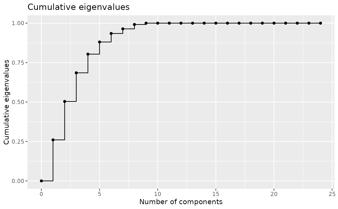
# plot eigenvalues
plotEigenvalues(encoding, cumulative = TRUE, normalize = TRUE)
 # modify the plot using ggplot2
library(ggplot2)
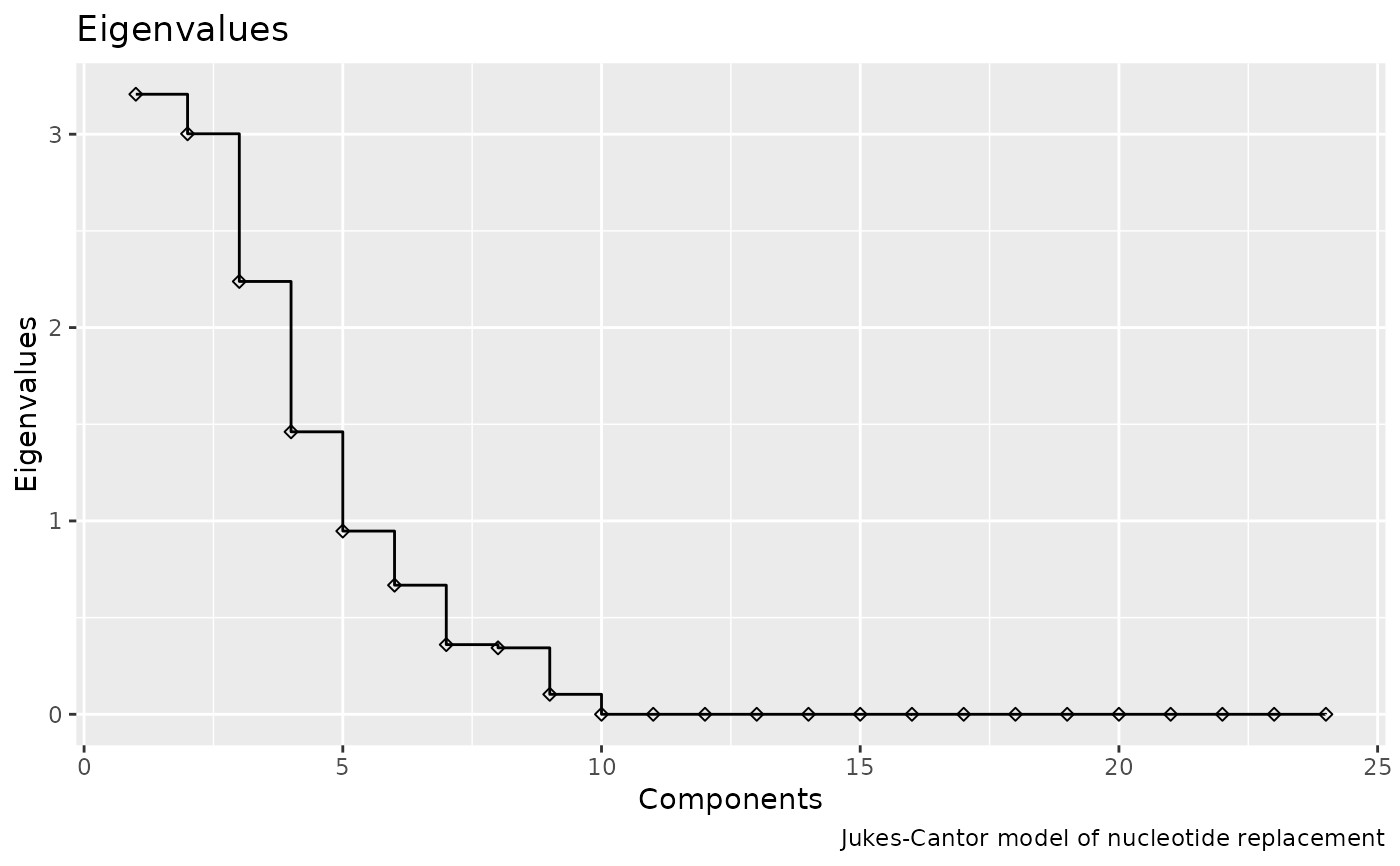
plotEigenvalues(encoding, shape = 23) +
labs(caption = "Jukes-Cantor model of nucleotide replacement")
# modify the plot using ggplot2
library(ggplot2)
plotEigenvalues(encoding, shape = 23) +
labs(caption = "Jukes-Cantor model of nucleotide replacement")
 # }
# }